4. Test simulations

These are a number of computationally rather inexpensive test simulations, of which the run-specs header files are contained in the SICOPOLIS repository.

Run repo_vialov3d25

3D version of the 2D Vialov profile (Vialov [59]),

SIA, resolution 25 km, \(t=0\ldots{}100\,\mathrm{ka}\).

Similar to the EISMINT Phase 1 fixed-margin experiment (Huybrechts et al. [41]), but without thermodynamics. Instead, isothermal conditions with \(T=-10^{\circ}\mathrm{C}\) everywhere are assumed.

Run repo_emtp2sge25_expA

EISMINT Phase 2 Simplified Geometry Experiment A,

SIA, resolution 25 km, \(t=0\ldots{}200\,\mathrm{ka}\) (Payne et al. [51]).

The thermodynamics solver for this run is the one-layer melting-CTS enthalpy scheme (ENTM), while all other runs employ the polythermal two-layer scheme (POLY) (Greve and Blatter [31]).

Run repo_grl16_bm5_ss25ka

Greenland ice sheet, SIA, resolution 16 km,

short steady-state run (\(t=0\ldots{}25\,\mathrm{ka}\)) for modern climate conditions (Fig. 4.1; unpublished).

Runs repo_grl16_bm5_{init100a, ss25ka_nudged}

Greenland ice sheet, SIA, resolution 16 km;

\(t=-100\,\mathrm{a}\ldots{}0\) for the init run without basal sliding (…_init100a),

\(t=0\,\ldots{}25\,\mathrm{ka}\) for the main run (…_ss25ka_nudged),

steady-state run for modern climate conditions, free evolution during the first 10 ka, after that gradual nudging towards the slightly smoothed present-day topography computed by the init run (Fig. 4.1; unpublished).

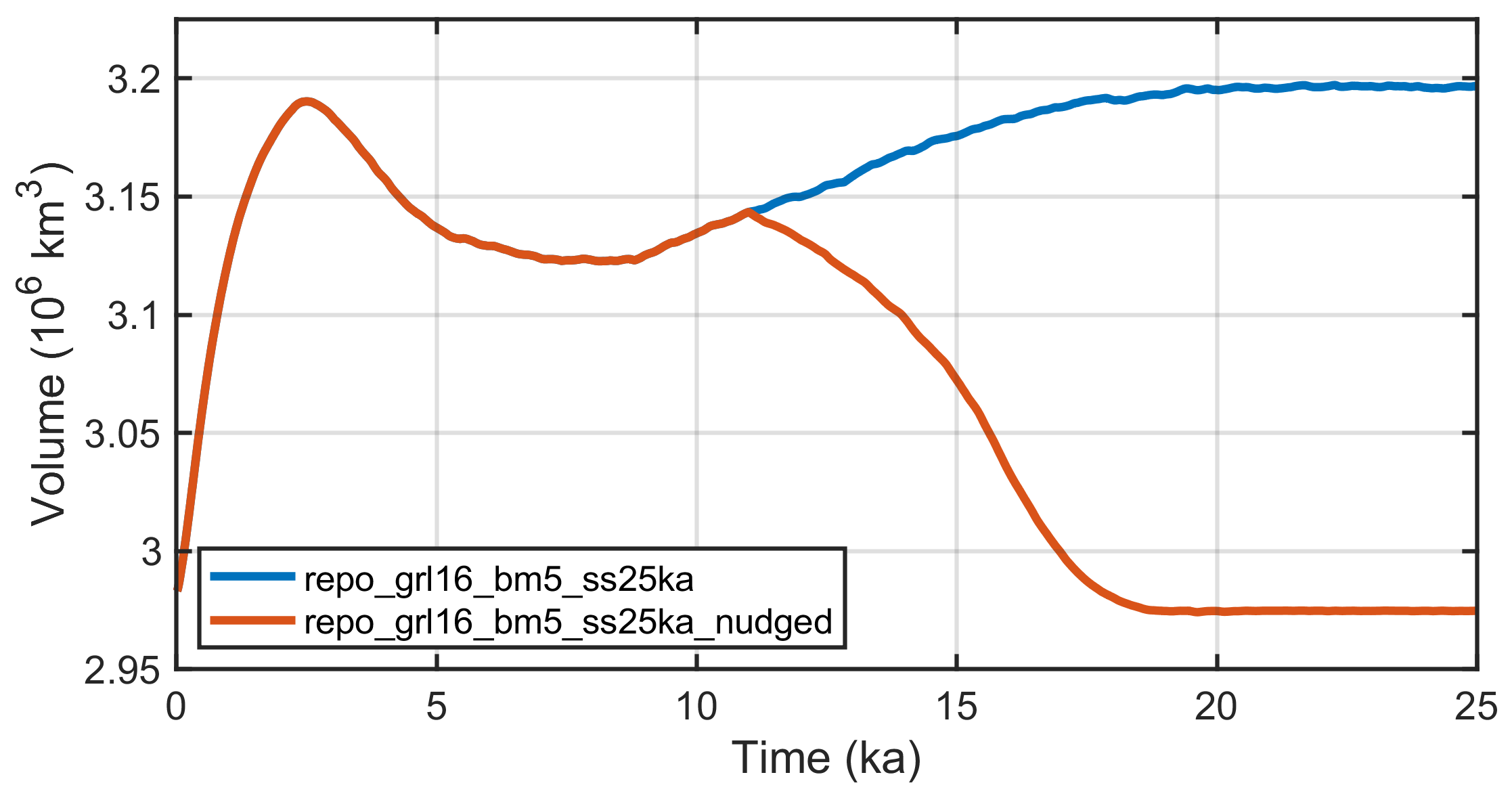
Fig. 4.1 Ice volume for the two steady-state simulations for Greenland, repo_grl16_bm5_ss25ka (unconstrained evolution) and repo_grl16_bm5_ss25ka_nudged (topography nudging with time-dependent relaxation time after t = 10 ka).

Run repo_ant64_bm3_ss25ka

Antarctic ice sheet, hybrid shallow-ice–shelfy-stream dynamics (Bernales et al. [5]),

instantaneous removal of ice shelves (“float-kill”), resolution 64 km,

short steady-state run (\(t=0\ldots{}25\,\mathrm{ka}\)) for modern climate conditions (Fig. 4.2; unpublished).

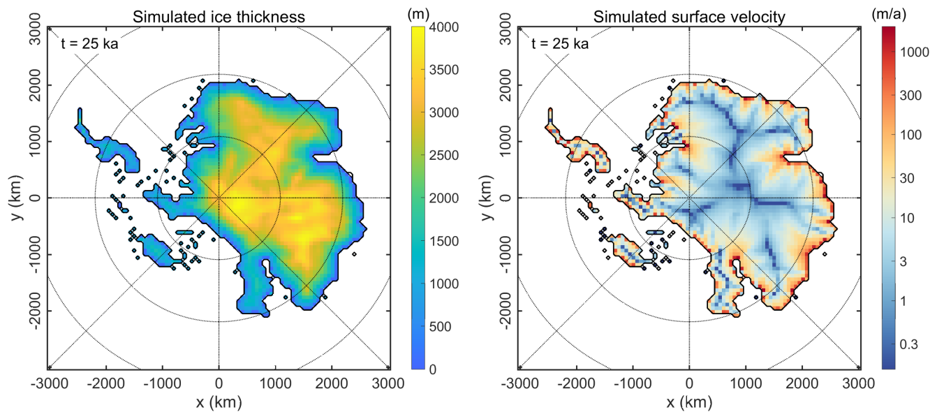
Fig. 4.2 Ice thickness and surface velocity for the short steady-state simulation for Antarctica with instantaneous removal of ice shelves (“float-kill”), repo_ant64_bm3_ss25ka. The West Antarctic ice sheet has largely disappeared.

Run repo_grl20_b2_paleo21

Greenland ice sheet, SIA, resolution 20 km,

\(t=-140\,\mathrm{ka}\ldots{}0\), basal sliding ramped up during the first 5 ka.

Modified, low-resolution version of the spin-up for ISMIP6 InitMIP (Greve et al. [33]).

Runs repo_grl10_b2_{paleo21, future21_ctrl, future21_asmb}

Greenland ice sheet, SIA, resolution 10 km,

\(t=-9\,\mathrm{ka}\ldots{}0\) for the paleo run, \(t=0\ldots{}100\,\mathrm{a}\) for the two future runs.

10-km version of the spin-up and schematic future climate runs for ISMIP6 InitMIP

(Fig. 4.3; Greve et al. [33], Seroussi et al. [57]).

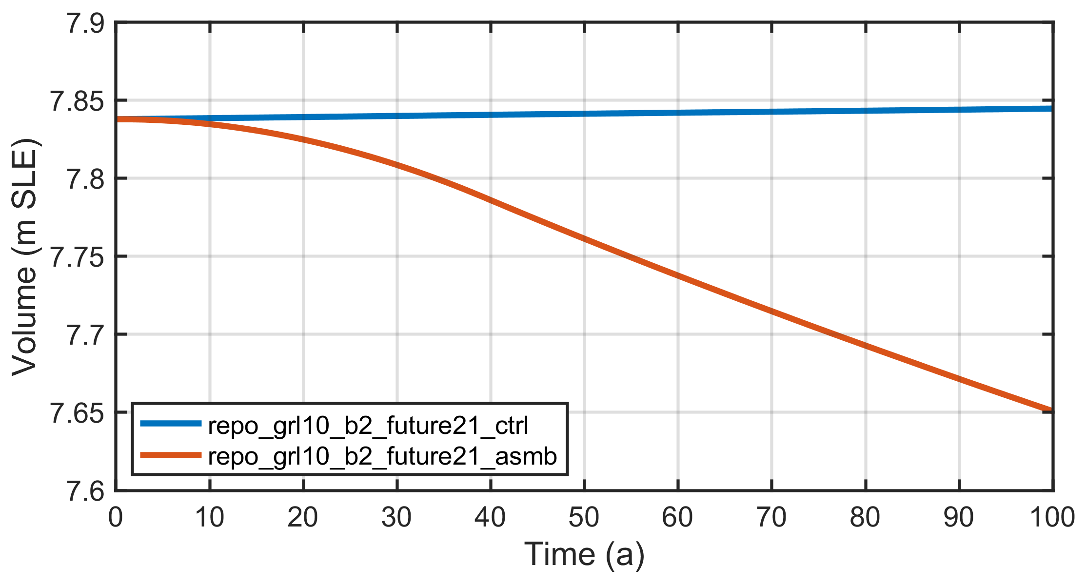
Fig. 4.3 Ice volume above flotation, expressed in metres of sea-level equivalent (m SLE), for the two ISMIP6 InitMIP future-climate simulations for Greenland, repo_grl10_b2_future21_ctrl (constant-climate control run) and repo_grl10_b2_future21_asmb (schematic surface-mass-balance anomaly applied).

Runs repo_ant64_b2_{spinup09_init100a, spinup09_fixtopo, spinup09, future09_ctrl, future09_asmb, future09_abmb}

Antarctic ice sheet with hybrid shallow-ice–shelfy-stream dynamics

(Bernales et al. [5]) and ice shelves (SSA), resolution 64 km;

\(t=-140.1\ldots{}-140\,\mathrm{ka}\) for the init run without basal sliding (…_init100a),

\(t=-140\,\mathrm{ka}\ldots{}0\) for the run with almost fixed topography (…_fixtopo), basal sliding ramped up during the first 5 ka,

\(t=-0.5\,\mathrm{ka}\ldots{}0\) for the final, freely-evolving-topography part of the spin-up (…_spinup09),

\(t=0\ldots{}100\,\mathrm{a}\) for the three future runs (…_future09_{ctrl, asmb, abmb}).

64-km version of the spin-up and schematic future climate runs for ISMIP6 InitMIP

(Fig. 4.4; Seroussi et al. [57]).

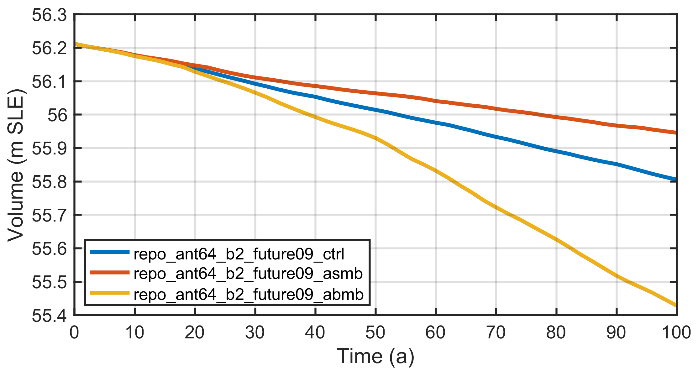
Fig. 4.4 Ice volume above flotation, expressed in metres of sea-level equivalent (m SLE), for the three ISMIP6 InitMIP future-climate simulations for Antarctica, repo_ant64_b2_future09_ctrl (constant-climate control run), repo_ant64_b2_future09_asmb (schematic surface-mass-balance anomaly applied) and repo_ant64_b2_future09_abmb (schematic sub-ice-shelf-melt anomaly applied).

Runs repo_asf2_steady, repo_asf2_surge

Austfonna, SIA, resolution 2 km, \(t=0\ldots{}10\,\mathrm{ka}\).

Similar to Dunse et al. [15]’s Exp. 2 (steady fast flow) and Exp. 5 (surging-type flow), respectively.

Runs repo_nmars10_steady, repo_smars10_steady

North-/south-polar cap of Mars, SIA, resolution 10 km, \(t=-10\,\mathrm{Ma}\ldots{}0\).

Steady-state runs by Greve [29].

Run repo_nhem80_nt012_new

Northern hemisphere, SIA, resolution 80 km, \(t=-250\,\mathrm{ka}\ldots{}0\).

Similar to run nt012 by Greve et al. [40].

Run repo_heino50_st

ISMIP HEINO standard run ST, SIA, resolution 50 km, \(t=0\ldots{}200\,\mathrm{ka}\) (Calov et al. [12]).

---

Model times, time steps, computing times:

Run	Model time	Time step†	CPU time‡
repo_vialov3d25	100 ka	20 a	1.0 min
repo_emtp2sge25_expA	200 ka	20 a	4.6 min
repo_grl16_bm5_ss25ka	25 ka	5 a	10.8 min
repo_grl16_bm5_init100a	100 a	5 a	1.6 sec
repo_grl16_bm5_ss25ka_nudged	25 ka	5 a	10.6 min
repo_ant64_bm3_ss25ka	25 ka	2 / 10 a†	8.9 min
repo_grl20_b2_paleo21	140 ka	5 a	0.9 hrs
repo_grl10_b2_paleo21*	9 ka	1 a	1.1 hrs
repo_grl10_b2_future21_ctrl	100 a	1 a	0.9 min
repo_grl10_b2_future21_asmb	100 a	1 a	0.9 min
repo_ant64_b2_spinup09_init100a	100 a	2 / 10 a†	4.3 sec
repo_ant64_b2_spinup09_fixtopo	140 ka	5 / 10 a†	0.7 hrs
repo_ant64_b2_spinup09	500 a	2 / 10 a†	0.5 min
repo_ant64_b2_future09_ctrl	100 a	2 / 10 a†	6.3 sec
repo_ant64_b2_future09_asmb	100 a	2 / 10 a†	6.3 sec
repo_ant64_b2_future09_abmb	100 a	2 / 10 a†	6.3 sec

Table 1: Model times, time steps and computing (CPU) times for the EISMINT, Greenland and Antarctica test simulations contained in the script multi_sico_1.sh, run with SICOPOLIS v23 (revision 1353323e2) and the Intel Fortran Compiler 19.1 for Linux (optimization options -xHOST -O3 -no-prec-div) on a 12-Core Intel Xeon Gold 6256 (3.6 GHz) PC under openSUSE Leap 15.5.

^†: If one value is given, this is the common dynamic (velocity, ice thickness) and thermodynamic (temperature, water content, age) time step. If two values are given (marked by the dagger (^†) symbol), the first one is the dynamic, the second one the thermodynamic time step.

^‡: All runs were done on a single core only. The repo_ant64_xxx runs can be done on multiple cores using OpenMP for the SSA solver. However, at the employed, low resolution of 64 km the solver does not scale well, and the gain in wall clock time by using multiple cores is very small.

^*: For this run, see the remark in the subsection on the resolution-doubler tool.