8.8.2. Tutorial 2: Using Tapenade for a mountain glacier model
In this tutorial, we will describe the steps to use Tapenade to develop the tangent linear and adjoint codes for a simple PDE-based mountain glacier model. The model itself is inspired from the book Fundamentals of Glacier Dynamics, by CJ van der Veen and has been used for glaciology summer schools before, for example here , although they used a different tool to develop the adjoint model.
As prerequisites, ensure you have Tapenade installed and gfortran compiler available.
8.8.2.1. Mountain glacier model
8.8.2.1.1. Model description
The equations for a simple, 1D mountain glacier are described here.
where
and
Here \(H(x,t)\) is the thickness of the ice sheet, \(h(x,t)\) is the height of the top surface of the ice sheet (taken from some reference height), \(b(x)\) is the height of the base of the ice sheet (taken from the same reference height). These three parameters can be related as
In essence it’s a highly non-linear diffusion equation with a source term. Furthermore, the boundary conditions are given by
and
8.8.2.1.2. Model parameters
We assume that the basal topography is linear in \(x\) such that \(\frac{\partial{b}}{\partial{x}} = -0.1\). \(M\) is the accumulation rate and is modeled to be constant in time, but varying linearly in space.
where \(M_0 = 4.0 \:{\rm m/yr}, \:M_1 = 0.0002 \:{\rm yr}^{-1}\).
The acceleration due to gravity \(g = 9.2 \:{\rm m/s}^2\). The density of ice \(\rho = 920 \:{\rm kg/m}^3\). The exponent \(n = 3\) comes from Glen’s flow law. We take \(A = 10^{-16} \: {\rm Pa}^{-3} {\rm a}^{-1}\). Our domain length is \(L = 30 \:{\rm km}\). The total time we run the simulation for is \(T = 5000 \:{\rm years}\).
8.8.2.1.3. Discretization and Finite Volumes solution
The equations above cannot be solved analytically. Here we discuss a Finite Volumes method to solve them. We use a staggered grid such that \(D\) is computed at the centres of the grid, and \(H, h\) are computed at the vertices.
Here, \(\phi\) indicates flux and is just an intermediate variable.
We step forward in time using the simple Euler forward scheme. Here we choose \(\Delta x = 1.0\:{\rm km}, \Delta t = 1.0\:{\rm month} = \frac{1}{12}\:{\rm years}\).
8.8.2.1.4. What sensitivities are we interested in?
Our Quantity of Interest (QoI) is the total volume of the ice sheet after 5000 years (defined as V in the code). The control variables are the spatially varying accumulation rate. We are interested in the sensitivities of the QoI to the perturbations in the accumulation rate at various locations along the ice sheet. (defined as xx in the code)
8.8.2.2. Forward Model code
The code for the non-linear forward model is given here.
forward.f90
module forward

implicit none
     real(8), parameter :: xend = 30
     real(8), parameter :: dx = 1
     integer, parameter :: nx = int(xend/dx)


contains

     subroutine forward_problem(xx,V)

             implicit none

             real(8), parameter :: rho = 920.0
             real(8), parameter :: g = 9.2
             real(8), parameter :: n = 3
             real(8), parameter :: A = 1e-16
             real(8), parameter :: dt = 1/12.0
             real(8), parameter :: C = 2*A/(n+2)*(rho*g)**n*(1.e3)**n
             real(8), parameter :: tend = 5000
             real(8), parameter :: bx = -0.0001
             real(8), parameter :: M0 = .004, M1 = 0.0002
             integer, parameter :: nt = int(tend/dt)
             real(8), dimension(nx+1,nt+1) :: h
             real(8), dimension(nx+1,nt+1) :: h_capital
             integer :: t,i
             real(8), dimension(nx+1) :: xarr
             real(8), dimension(nx+1) :: M
             real(8), dimension(nx+1) :: b
             real(8), dimension(nx) :: D, phi
             real(8), intent(in), dimension(nx+1) :: xx
             real(8), intent(out) :: V

             xarr = (/ ((i-1)*dx, i=1,nx+1) /)
             M = (/ (M0-(i-1)*dx*M1, i=1,nx+1) /)
             b = (/ (1.0+bx*(i-1)*dx, i=1,nx+1) /)
             M = M + xx
             h(1,:) = b(1)
             h(:,1) = b
             h(nx+1,:) = b(nx+1)
             h_capital(1,:) = h(1,:) - b(1)
             h_capital(nx+1,:) = h(nx+1,:) - b(nx+1)
             h_capital(:,1) = h(:,1) - b

             do t = 1,nt
                     D(:) = C * ((h_capital(1:nx,t)+h_capital(2:nx+1,t))/2)**(n+2) * ((h(2:nx+1,t) - h(1:nx,t))/dx)**(n-1)
                     phi(:) = -D(:)*(h(2:nx+1,t)-h(1:nx,t))/dx
                     h(2:nx,t+1) = h(2:nx,t) + M(2:nx)*dt - dt/dx * (phi(2:nx)-phi(1:nx-1))

                     where (h(:,t+1) < b)
                             h(:,t+1) = b
                     end where

                     h_capital(:,t+1) = h(:,t+1) - b

             end do

             V = 0.


             open (unit = 2, file = "results_forward_run.txt", action="write",status="replace")
             write(2,*) "         #                H                h                  b"
             write(2,*) "_______________________________________________________________________________"

             do i = 1, size(h_capital(:,nt+1))
                  V = V + h_capital(i,nt+1)*dx

                  write(2,*) i, "    ", h_capital(i,nt+1), "    ", h(i,nt+1), "    ", b(i)
             end do


     close(2)
     end subroutine forward_problem

end module forward
8.8.2.3. Finite Differences for validation
We can use finite differences with the forward differencing scheme (or alternatively, a more accurate central differencing scheme mentioned in Tutorial 1 ). to get the gradient evaluated at the given value of the control vector \(\mathbf{x}\). For a \(N\) dimensional control vector, the forward model needs to be called \(N+1\) times in the forward differencing scheme to get an approximate gradient. This is because we can only evaluate directional derivatives, which we need to do \(N\) times to get the gradient. Each directional derivative evaluation, in turn, requires 1 perturbed forward model evaluation and 1 unperturbed forward model evaluation (this can be done only once and stored).
Mathematically, this can be formulated as (\(\mathcal{J}\) is the objective function, in our case the total volume denoted by V in the code)
Here \((.,.)\) indicates the normal inner product of two discrete vectors in \(\mathbb{R}^N\).
The left side is the directional derivative of \(\mathcal{J}\) at \(\mathbf{x}\) in the direction \(\hat{\mathbf{e}}\), while the right side is the finite differences approximation of the directional derivative.
The choice of \(\epsilon\) can be critical, however we do not discuss that here and simply choose a value \(\epsilon = 1.e-7\). In general, one would perform a convergence analysis with a range of values of \(\epsilon = {0.1, 0.01, 0.001, ...}\).
The code for the finite differences can be found in the Driver Routine.
8.8.2.4. Tangent Linear model
The tangent linear model is described in detail in Tutorial 1. Another excellent resource is the MITgcm documentation.
8.8.2.4.1. Generating Tangent Linear model code using Tapenade
It is pretty simple to generate the tangent linear model for our forward model.
% tapenade -tangent -tgtmodulename %_tgt -head "forward_problem(V)/(xx)" forward.f90
-tangent tells Tapenade that we want a tangent linear code.
-tgtmodulename %_tgt tells Tapenade to suffix the differentiated modules with _tgt.
-head "forward_problem(V)/(xx) tells Tapenade that the head subroutine is forward_problem, the dependent variable or the objective function is V and the independent variable is xx.
This generates 2 files -
forward_d.f90- This file contains the tangent linear module (calledforward_tgt) as well as the original forward code module.forward_tgt) contains theforward_problem_dsubroutine which is our tangent linear model. All the differential variables are suffixed with the alphabetd.
!        Generated by TAPENADE     (INRIA, Ecuador team)
!  TAPENADE 3.15 (master) - 15 Apr 2020 13:12
!
MODULE FORWARD_TGT
  IMPLICIT NONE
  REAL*8, PARAMETER :: xend=30
  REAL*8, PARAMETER :: dx=1
  INTEGER, PARAMETER :: nx=INT(xend/dx)

CONTAINS
!  Differentiation of forward_problem in forward (tangent) mode:
!   variations   of useful results: v
!   with respect to varying inputs: xx
!   RW status of diff variables: v:out xx:in
  SUBROUTINE FORWARD_PROBLEM_D(xx, xxd, v, vd)
    IMPLICIT NONE
    REAL*8, PARAMETER :: rho=920.0
    REAL*8, PARAMETER :: g=9.2
    REAL*8, PARAMETER :: n=3
    REAL*8, PARAMETER :: a=1e-16
    REAL*8, PARAMETER :: dt=1/12.0
    REAL*8, PARAMETER :: c=2*a/(n+2)*(rho*g)**n*1.e3**n
    REAL*8, PARAMETER :: tend=5000
    REAL*8, PARAMETER :: bx=-0.0001
    REAL*8, PARAMETER :: m0=.004, m1=0.0002
    INTRINSIC INT
    INTEGER, PARAMETER :: nt=INT(tend/dt)
    REAL*8, DIMENSION(nx+1, nt+1) :: h
    REAL*8, DIMENSION(nx+1, nt+1) :: hd
    REAL*8, DIMENSION(nx+1, nt+1) :: h_capital
    REAL*8, DIMENSION(nx+1, nt+1) :: h_capitald
    INTEGER :: t, i
    REAL*8, DIMENSION(nx+1) :: xarr
    REAL*8, DIMENSION(nx+1) :: m
    REAL*8, DIMENSION(nx+1) :: md
    REAL*8, DIMENSION(nx+1) :: b
    REAL*8, DIMENSION(nx) :: d, phi
    REAL*8, DIMENSION(nx) :: dd, phid
    REAL*8, DIMENSION(nx+1), INTENT(IN) :: xx
    REAL*8, DIMENSION(nx+1), INTENT(IN) :: xxd
    REAL*8, INTENT(OUT) :: v
    REAL*8, INTENT(OUT) :: vd
    INTRINSIC SIZE
    REAL*8, DIMENSION(nx) :: pwx1
    REAL*8, DIMENSION(nx) :: pwx1d
    REAL*8 :: pwy1
    REAL*8, DIMENSION(nx) :: pwr1
    REAL*8, DIMENSION(nx) :: pwr1d
    REAL*8, DIMENSION(nx) :: pwx2
    REAL*8, DIMENSION(nx) :: pwx2d
    REAL*8 :: pwy2
    REAL*8, DIMENSION(nx) :: pwr2
    REAL*8, DIMENSION(nx) :: pwr2d
    REAL*8, DIMENSION(nx) :: temp
    xarr = (/((i-1)*dx, i=1,nx+1)/)
    m = (/(m0-(i-1)*dx*m1, i=1,nx+1)/)
    b = (/(1.0+bx*(i-1)*dx, i=1,nx+1)/)
    md = xxd
    m = m + xx
    h(1, :) = b(1)
    h(:, 1) = b
    h(nx+1, :) = b(nx+1)
    h_capital(1, :) = h(1, :) - b(1)
    h_capital(nx+1, :) = h(nx+1, :) - b(nx+1)
    h_capital(:, 1) = h(:, 1) - b
    h_capitald = 0.0_8
    hd = 0.0_8
    DO t=1,nt
      pwx1d = (h_capitald(1:nx, t)+h_capitald(2:nx+1, t))/2
      pwx1 = (h_capital(1:nx, t)+h_capital(2:nx+1, t))/2
      pwy1 = n + 2
      WHERE (pwx1 .LE. 0.0 .AND. (pwy1 .EQ. 0.0 .OR. pwy1 .NE. INT(pwy1)&
&         ))
        pwr1d = 0.0_8
      ELSEWHERE
        pwr1d = pwy1*pwx1**(pwy1-1)*pwx1d
      END WHERE
      pwr1 = pwx1**pwy1
      pwx2d = (hd(2:nx+1, t)-hd(1:nx, t))/dx
      pwx2 = (h(2:nx+1, t)-h(1:nx, t))/dx
      pwy2 = n - 1
      WHERE (pwx2 .LE. 0.0 .AND. (pwy2 .EQ. 0.0 .OR. pwy2 .NE. INT(pwy2)&
&         ))
        pwr2d = 0.0_8
      ELSEWHERE
        pwr2d = pwy2*pwx2**(pwy2-1)*pwx2d
      END WHERE
      pwr2 = pwx2**pwy2
      dd(:) = c*(pwr2*pwr1d+pwr1*pwr2d)
      d(:) = c*pwr1*pwr2
      temp = h(2:nx+1, t) - h(1:nx, t)
      phid(:) = -(temp*dd(:)/dx+d(:)*(hd(2:nx+1, t)-hd(1:nx, t))/dx)
      phi(:) = -(d(:)/dx*temp)
      hd(2:nx, t+1) = hd(2:nx, t) + dt*md(2:nx) - dt*(phid(2:nx)-phid(1:&
&       nx-1))/dx
      h(2:nx, t+1) = h(2:nx, t) + m(2:nx)*dt - dt/dx*(phi(2:nx)-phi(1:nx&
&       -1))
      WHERE (h(:, t+1) .LT. b)
        hd(:, t+1) = 0.0_8
        h(:, t+1) = b
      END WHERE
      h_capitald(:, t+1) = hd(:, t+1)
      h_capital(:, t+1) = h(:, t+1) - b
    END DO
    v = 0.
    OPEN(unit=2, file='results_forward_run.txt', action='write', status=&
&  'replace')
    WRITE(2, *) &
&   '         #                H                h                  b'
    WRITE(2, *) '_______________________________________________________&
&________________________'
    vd = 0.0_8
    DO i=1,SIZE(h_capital(:, nt+1))
      vd = vd + dx*h_capitald(i, nt+1)
      v = v + h_capital(i, nt+1)*dx
      WRITE(2, *) i, '    ', h_capital(i, nt+1), '    ', h(i, nt+1), &
&     '    ', b(i)
    END DO
    CLOSE(2)
  END SUBROUTINE FORWARD_PROBLEM_D

  SUBROUTINE FORWARD_PROBLEM(xx, v)
    IMPLICIT NONE
    REAL*8, PARAMETER :: rho=920.0
    REAL*8, PARAMETER :: g=9.2
    REAL*8, PARAMETER :: n=3
    REAL*8, PARAMETER :: a=1e-16
    REAL*8, PARAMETER :: dt=1/12.0
    REAL*8, PARAMETER :: c=2*a/(n+2)*(rho*g)**n*1.e3**n
    REAL*8, PARAMETER :: tend=5000
    REAL*8, PARAMETER :: bx=-0.0001
    REAL*8, PARAMETER :: m0=.004, m1=0.0002
    INTRINSIC INT
    INTEGER, PARAMETER :: nt=INT(tend/dt)
    REAL*8, DIMENSION(nx+1, nt+1) :: h
    REAL*8, DIMENSION(nx+1, nt+1) :: h_capital
    INTEGER :: t, i
    REAL*8, DIMENSION(nx+1) :: xarr
    REAL*8, DIMENSION(nx+1) :: m
    REAL*8, DIMENSION(nx+1) :: b
    REAL*8, DIMENSION(nx) :: d, phi
    REAL*8, DIMENSION(nx+1), INTENT(IN) :: xx
    REAL*8, INTENT(OUT) :: v
    INTRINSIC SIZE
    REAL*8, DIMENSION(nx) :: pwx1
    REAL*8 :: pwy1
    REAL*8, DIMENSION(nx) :: pwr1
    REAL*8, DIMENSION(nx) :: pwx2
    REAL*8 :: pwy2
    REAL*8, DIMENSION(nx) :: pwr2
    xarr = (/((i-1)*dx, i=1,nx+1)/)
    m = (/(m0-(i-1)*dx*m1, i=1,nx+1)/)
    b = (/(1.0+bx*(i-1)*dx, i=1,nx+1)/)
    m = m + xx
    h(1, :) = b(1)
    h(:, 1) = b
    h(nx+1, :) = b(nx+1)
    h_capital(1, :) = h(1, :) - b(1)
    h_capital(nx+1, :) = h(nx+1, :) - b(nx+1)
    h_capital(:, 1) = h(:, 1) - b
    DO t=1,nt
      pwx1 = (h_capital(1:nx, t)+h_capital(2:nx+1, t))/2
      pwy1 = n + 2
      pwr1 = pwx1**pwy1
      pwx2 = (h(2:nx+1, t)-h(1:nx, t))/dx
      pwy2 = n - 1
      pwr2 = pwx2**pwy2
      d(:) = c*pwr1*pwr2
      phi(:) = -(d(:)*(h(2:nx+1, t)-h(1:nx, t))/dx)
      h(2:nx, t+1) = h(2:nx, t) + m(2:nx)*dt - dt/dx*(phi(2:nx)-phi(1:nx&
&       -1))
      WHERE (h(:, t+1) .LT. b) h(:, t+1) = b
      h_capital(:, t+1) = h(:, t+1) - b
    END DO
    v = 0.
    OPEN(unit=2, file='results_forward_run.txt', action='write', status=&
&  'replace')
    WRITE(2, *) &
&   '         #                H                h                  b'
    WRITE(2, *) '_______________________________________________________&
&________________________'
    DO i=1,SIZE(h_capital(:, nt+1))
      v = v + h_capital(i, nt+1)*dx
      WRITE(2, *) i, '    ', h_capital(i, nt+1), '    ', h(i, nt+1), &
&     '    ', b(i)
    END DO
    CLOSE(2)
  END SUBROUTINE FORWARD_PROBLEM

END MODULE FORWARD_TGT
forward_d.msg- Contains warning messages. TAPENADE can be quite verbose with the warnings. None of the warnings below are much important.
1 Command: Procedure forward_problem understood as forward.forward_problem
2 forward_problem: (AD03) Varied variable h[i,nt+1] written by I-O to file 2
3 forward_problem: (AD03) Varied variable h_capital[i,nt+1] written by I-O to file 2
~
8.8.2.5. Adjoint Model
The adjoint model is described in detail in Tutorial 1. Another excellent resource is the MITgcm documentation.
8.8.2.5.1. Generating Adjoint model code using Tapenade
It is pretty simple to generate the tangent linear model for our forward model.
% tapenade -reverse -head "forward_problem(V)/(xx)" forward.f90
-reverse tells Tapenade that we want a reverse i.e. adjoint code.
-head "forward_problem(V)/(xx) tells Tapenade that the head subroutine is forward_problem, the dependent variable or the objective function is V and the independent variable is xx.
This generates 2 files -
forward_b.f90- This file contains the adjoint module (calledforward_diff) as well as the original forward code module.forward_diffcontains theforward_problem_bsubroutine which is our adjoint model. Notice how it requires values forxx, Vwhich have to be obtained from a forward solve (calling theforwardsubroutine). We also will defineVb = 1and propagate the adjoint sensitivities backwards to evaluatexxb. If you look at the secondDOloop inforward_problem_b, it indeed runs backwards in time. Note that all the adjoint variables in the code are simply suffixed with the alphabetb. There are also a lot ofPUSHandPOPstatements, they are essentially pushing and popping the stored variables from a stack just like we did manually in Tutorial 1.
!  TAPENADE 3.15 (master) - 15 Apr 2020 13:12
!
MODULE FORWARD_DIFF
  IMPLICIT NONE
  REAL*8, PARAMETER :: xend=30
  REAL*8, PARAMETER :: dx=1
  INTEGER, PARAMETER :: nx=INT(xend/dx)

CONTAINS
!  Differentiation of forward_problem in reverse (adjoint) mode:
!   gradient     of useful results: v
!   with respect to varying inputs: v xx
!   RW status of diff variables: v:in-zero xx:out
  SUBROUTINE FORWARD_PROBLEM_B(xx, xxb, v, vb)
    IMPLICIT NONE
    REAL*8, PARAMETER :: rho=920.0
    REAL*8, PARAMETER :: g=9.2
    REAL*8, PARAMETER :: n=3
    REAL*8, PARAMETER :: a=1e-16
    REAL*8, PARAMETER :: dt=1/12.0
    REAL*8, PARAMETER :: c=2*a/(n+2)*(rho*g)**n*1.e3**n
    REAL*8, PARAMETER :: tend=5000
    REAL*8, PARAMETER :: bx=-0.0001
    REAL*8, PARAMETER :: m0=.004, m1=0.0002
    INTRINSIC INT
    INTEGER, PARAMETER :: nt=INT(tend/dt)
    REAL*8, DIMENSION(nx+1, nt+1) :: h
    REAL*8, DIMENSION(nx+1, nt+1) :: hb
    REAL*8, DIMENSION(nx+1, nt+1) :: h_capital
    REAL*8, DIMENSION(nx+1, nt+1) :: h_capitalb
    INTEGER :: t, i
    REAL*8, DIMENSION(nx+1) :: xarr
    REAL*8, DIMENSION(nx+1) :: m
    REAL*8, DIMENSION(nx+1) :: mb
    REAL*8, DIMENSION(nx+1) :: b
    REAL*8, DIMENSION(nx) :: d, phi
    REAL*8, DIMENSION(nx) :: db, phib
    REAL*8, DIMENSION(nx+1), INTENT(IN) :: xx
    REAL*8, DIMENSION(nx+1) :: xxb
    REAL*8 :: v
    REAL*8 :: vb
    INTRINSIC SIZE
    LOGICAL, DIMENSION(nx+1) :: mask
    REAL*8, DIMENSION(nx) :: temp
    REAL*8, DIMENSION(nx) :: temp0
    REAL*8, DIMENSION(nx) :: tempb
    REAL*8, DIMENSION(nx) :: tempb0
    REAL*8, DIMENSION(nx-1) :: tempb1
    INTEGER :: ad_to
    m = (/(m0-(i-1)*dx*m1, i=1,nx+1)/)
    b = (/(1.0+bx*(i-1)*dx, i=1,nx+1)/)
    m = m + xx
    h(1, :) = b(1)
    h(:, 1) = b
    h(nx+1, :) = b(nx+1)
    h_capital(1, :) = h(1, :) - b(1)
    h_capital(nx+1, :) = h(nx+1, :) - b(nx+1)
    h_capital(:, 1) = h(:, 1) - b
    DO t=1,nt
      CALL PUSHREAL8ARRAY(d, nx)
      d(:) = c*((h_capital(1:nx, t)+h_capital(2:nx+1, t))/2)**(n+2)*((h(&
&       2:nx+1, t)-h(1:nx, t))/dx)**(n-1)
      phi(:) = -(d(:)*(h(2:nx+1, t)-h(1:nx, t))/dx)
      CALL PUSHREAL8ARRAY(h(2:nx, t+1), nx - 1)
      h(2:nx, t+1) = h(2:nx, t) + m(2:nx)*dt - dt/dx*(phi(2:nx)-phi(1:nx&
&       -1))
      CALL PUSHBOOLEANARRAY(mask, nx + 1)
      mask(:) = h(:, t+1) .LT. b
      CALL PUSHREAL8ARRAY(h(:, t+1), nx + 1)
      WHERE (mask(:)) h(:, t+1) = b
      CALL PUSHREAL8ARRAY(h_capital(:, t+1), nx + 1)
      h_capital(:, t+1) = h(:, t+1) - b
    END DO
    DO i=1,SIZE(h_capital(:, nt+1))

    END DO
    CALL PUSHINTEGER4(i - 1)
    h_capitalb = 0.0_8
    CALL POPINTEGER4(ad_to)
    DO i=ad_to,1,-1
      h_capitalb(i, nt+1) = h_capitalb(i, nt+1) + dx*vb
    END DO
    hb = 0.0_8
    mb = 0.0_8
    DO t=nt,1,-1
      CALL POPREAL8ARRAY(h_capital(:, t+1), nx + 1)
      hb(:, t+1) = hb(:, t+1) + h_capitalb(:, t+1)
      h_capitalb(:, t+1) = 0.0_8
      CALL POPREAL8ARRAY(h(:, t+1), nx + 1)
      CALL POPBOOLEANARRAY(mask, nx + 1)
      phib = 0.0_8
      CALL POPREAL8ARRAY(h(2:nx, t+1), nx - 1)
      db = 0.0_8
      temp = (h(2:nx+1, t)-h(1:nx, t))/dx
      temp0 = (h_capital(1:nx, t)+h_capital(2:nx+1, t))/2
      WHERE (mask(:)) hb(:, t+1) = 0.0_8
      hb(2:nx, t) = hb(2:nx, t) + hb(2:nx, t+1)
      mb(2:nx) = mb(2:nx) + dt*hb(2:nx, t+1)
      tempb1 = -(dt*hb(2:nx, t+1)/dx)
      hb(2:nx, t+1) = 0.0_8
      phib(2:nx) = phib(2:nx) + tempb1
      phib(1:nx-1) = phib(1:nx-1) - tempb1
      db(:) = -((h(2:nx+1, t)-h(1:nx, t))*phib(:)/dx)
      tempb = -(d(:)*phib(:)/dx)
      hb(2:nx+1, t) = hb(2:nx+1, t) + tempb
      hb(1:nx, t) = hb(1:nx, t) - tempb
      CALL POPREAL8ARRAY(d, nx)
      WHERE (temp0 .LE. 0.0 .AND. (n + 2 .EQ. 0.0 .OR. n + 2 .NE. INT(n &
&         + 2)))
        tempb = 0.0_8
      ELSEWHERE
        tempb = (n+2)*temp0**(n+1)*temp**(n-1)*c*db(:)/2
      END WHERE
      WHERE (temp .LE. 0.0 .AND. (n - 1 .EQ. 0.0 .OR. n - 1 .NE. INT(n -&
&         1)))
        tempb0 = 0.0_8
      ELSEWHERE
        tempb0 = (n-1)*temp**(n-2)*temp0**(n+2)*c*db(:)/dx
      END WHERE
      hb(2:nx+1, t) = hb(2:nx+1, t) + tempb0
      hb(1:nx, t) = hb(1:nx, t) - tempb0
      h_capitalb(1:nx, t) = h_capitalb(1:nx, t) + tempb
      h_capitalb(2:nx+1, t) = h_capitalb(2:nx+1, t) + tempb
    END DO
    xxb = 0.0_8
    xxb = mb
    vb = 0.0_8
  END SUBROUTINE FORWARD_PROBLEM_B

  SUBROUTINE FORWARD_PROBLEM(xx, v)
    IMPLICIT NONE
    REAL*8, PARAMETER :: rho=920.0
    REAL*8, PARAMETER :: g=9.2
    REAL*8, PARAMETER :: n=3
    REAL*8, PARAMETER :: a=1e-16
    REAL*8, PARAMETER :: dt=1/12.0
    REAL*8, PARAMETER :: c=2*a/(n+2)*(rho*g)**n*1.e3**n
    REAL*8, PARAMETER :: tend=5000
    REAL*8, PARAMETER :: bx=-0.0001
    REAL*8, PARAMETER :: m0=.004, m1=0.0002
    INTRINSIC INT
    INTEGER, PARAMETER :: nt=INT(tend/dt)
    REAL*8, DIMENSION(nx+1, nt+1) :: h
    REAL*8, DIMENSION(nx+1, nt+1) :: h_capital
    INTEGER :: t, i
    REAL*8, DIMENSION(nx+1) :: xarr
    REAL*8, DIMENSION(nx+1) :: m
    REAL*8, DIMENSION(nx+1) :: b
    REAL*8, DIMENSION(nx) :: d, phi
    REAL*8, DIMENSION(nx+1), INTENT(IN) :: xx
    REAL*8, INTENT(OUT) :: v
    INTRINSIC SIZE
    LOGICAL, DIMENSION(nx+1) :: mask
    xarr = (/((i-1)*dx, i=1,nx+1)/)
    m = (/(m0-(i-1)*dx*m1, i=1,nx+1)/)
    b = (/(1.0+bx*(i-1)*dx, i=1,nx+1)/)
    m = m + xx
    h(1, :) = b(1)
    h(:, 1) = b
    h(nx+1, :) = b(nx+1)
    h_capital(1, :) = h(1, :) - b(1)
    h_capital(nx+1, :) = h(nx+1, :) - b(nx+1)
    h_capital(:, 1) = h(:, 1) - b
    DO t=1,nt
      d(:) = c*((h_capital(1:nx, t)+h_capital(2:nx+1, t))/2)**(n+2)*((h(&
&       2:nx+1, t)-h(1:nx, t))/dx)**(n-1)
      phi(:) = -(d(:)*(h(2:nx+1, t)-h(1:nx, t))/dx)
      h(2:nx, t+1) = h(2:nx, t) + m(2:nx)*dt - dt/dx*(phi(2:nx)-phi(1:nx&
&       -1))
      mask(:) = h(:, t+1) .LT. b
      WHERE (mask(:)) h(:, t+1) = b
      h_capital(:, t+1) = h(:, t+1) - b
    END DO
    v = 0.
    OPEN(unit=2, file='results_forward_run.txt', action='write', status=&
&  'replace')
    WRITE(2, *) &
&   '         #                H                h                  b'
    WRITE(2, *) '_______________________________________________________&
&________________________'
    DO i=1,SIZE(h_capital(:, nt+1))
      v = v + h_capital(i, nt+1)*dx
      WRITE(2, *) i, '    ', h_capital(i, nt+1), '    ', h(i, nt+1), &
&     '    ', b(i)
    END DO
    CLOSE(2)
  END SUBROUTINE FORWARD_PROBLEM

END MODULE FORWARD_DIFF
forward_b.msg- Contains warning messages. Tapenade can be quite verbose with the warnings. None of the warnings below are much important.
1 Command: Procedure forward_problem understood as forward.forward_problem
2 forward_problem: Command: Input variable(s) v have their derivative modified in forward_problem: added to independents
3 forward_problem: (AD03) Varied variable h[i,nt+1] written by I-O to file 2
4 forward_problem: (AD03) Varied variable h_capital[i,nt+1] written by I-O to file 2
8.8.2.6. Driver Routine
The driver routine evaluates the sensitivities of our cost function V to the independent variable xx in three ways - Finite Differences, Tangent Linear Model (forward mode), Adjoint Model (reverse mode). Both the TLM and adjoint methods should give sensitivities that agree within some tolerance with the Finite Differences sensitivities. One can see that the TLM and finite differences have to be called multiple times (as many times as the number of control variables) while the adjoint model only has to be called once to evaluate the entire gradient, making it much more efficient.
program driver
     !!Essentially both modules had variables with the same name
     !!so they had to be locally aliased for the code to compile and run
     !!Obviously only one set of variables is needed so the other is useless

     use forward_diff, n => nx, fp => forward_problem !! Alias to a local variable
     use forward_tgt, n_useless => nx, fp_useless => forward_problem

     implicit none

     real(8), dimension(n+1) :: xx=0., xx_tlm =0., xxb =0., xx_fd, accuracy
     real(8) :: V=0., Vb = 1., V_forward, Vd = 0.
     real(8), parameter :: eps = 1.d-7
     integer :: ii

     call fp(xx,V)

     !! Forward run
     V_forward = V


     !! Adjoint run
     xx = 0.
     V = 0.
     call fp(xx,V)
     call forward_problem_b(xx,xxb,V,Vb)


     open (unit = 1, file = "results.txt", action="write",status="replace")

     write(1,*) "         #                Reverse                           FD",&
                     "                          Tangent                     Relative accuracy"
     write(1,*) "______________________________________________________________",&
                     "_______________________________________________________________________"

     !! Finite differences and Tangent Linear Model
     do ii = 1, n+1

             xx = 0.
             V = 0.
             xx_tlm = 0.
             xx_tlm(ii) = 1.

             !! TLM
             call fp(xx,V)
             call forward_problem_d(xx,xx_tlm,V,Vd)


             !! FD
             xx = 0.
             V = 0.
             xx(ii) = eps
             call fp(xx,V)
             xx_fd(ii) =  (V - V_forward)/eps

        if ( xx_fd(ii).NE. 0. ) then
            accuracy(ii) = 1.d0 - Vd/xx_fd(ii)
        else
            accuracy(ii) = 0.
        end if
        write(1,*) ii, "    ", xxb(ii), "    ", xx_fd(ii),"    ", Vd,"    ", accuracy(ii)
     end do

     close(1)

     call execute_command_line('gnuplot plot.script')
end program driver
8.8.2.7. Combining all compilation commands into a Makefile
Makefiles are extremely useful to automate the compilation process. The Makefile shown below generates both the tangent linear and adjoint codes, and bundles everything together with the driver routine and a special file provided by the Tapenade developers, called adStack.c together into a single executable named adjoint (unfortunately, a slight misnomer since it also executes FD and TLM codes). adStack.c contains the definitions of the POP, PUSH mechanisms that Tapenade uses in its generated codes.
The adStack.c file can be found in test_ad/tapenade_supported/ADFirstAidKit sub-directory in the ad branch of the SICOPOLIS repository. The Makefile assumes that you have the entire ADFirstAidKit directory present, so it is better to copy the entire directory to work as is with this Makefile.
More information on Makefiles can be found here . Makefiles are extremely sensitive to whitespaces both at the start and end of any line, so you should be very careful with that.
Makefile:
EXEC := adjoint
SRC  := $(wildcard *.f90)
OBJ  := $(patsubst %.f90, %.o, $(SRC))
# NOTE - OBJ will not have the object files of c codes in it, this needs to be improved upon.
# Options
F90  := gfortran
CC           := gcc
TAP_AD_kit:= ./ADFirstAidKit

# Rules

$(EXEC): $(OBJ) adStack.o forward_b.o forward_d.o
             $(F90) -o $@ $^

%.o: %.f90
             $(F90) -c $<

driver.o: forward_b.f90 forward_diff.mod forward_tgt.mod
forward_diff.mod: forward_b.o
forward_tgt.mod: forward_d.o

adStack.o :
             $(CC) -c $(TAP_AD_kit)/adStack.c

forward_b.f90: forward.f90
             tapenade -reverse -head "forward_problem(V)/(xx)" forward.f90
forward_d.f90: forward.f90
             tapenade -tangent -tgtmodulename %_tgt -head "forward_problem(V)/(xx)" forward.f90
# Useful phony targets

.PHONY: clean

clean:
     $(RM) $(EXEC) *.o $(MOD) $(MSG) *.msg *.mod *_db.f90 *_b.f90 *_d.f90 *~
To compile everything, just type -
% make
To clean up the compilation, just type -
% make clean
8.8.2.8. Results
The results are shown here. The adjoint and the tangent linear model agree with each other up to 12 decimal places in most cases. The agreement of both of these with the Finite differences is also extremely good, as seen from the Relative accuracy.
         #                Reverse                           FD                          Tangent                     Relative accuracy
_____________________________________________________________________________________________________________________________________
          1        0.0000000000000000             0.0000000000000000             0.0000000000000000             0.0000000000000000
          2        7.7234861280779530             7.7234756545863092             7.7234861280783651            -1.3560594380734869E-006
          3        13.803334061615192             13.803310956461701             13.803334061616136            -1.6738849475395057E-006
          4        19.668654270913329             19.668613369105969             19.668654270914736            -2.0795471444845504E-006
          5        25.460720864192346             25.460657031572964             25.460720864194293            -2.5071081728444966E-006
          6        31.276957320291768             31.276862468843092             31.276957320293935            -3.0326395730195799E-006
          7        37.209906557896431             37.209769434554119             37.209906557899728            -3.6851436515661362E-006
          8        43.370516019133923             43.370320437219334             43.370516019138648            -4.5095797620575695E-006
          9        49.919848601374966             49.919570930256896             49.919848601380266            -5.5623699923845749E-006
         10        57.138817544000176             57.138414888413536             57.138817544006628            -7.0470207107486971E-006
         11        65.642858080405333             65.642249307273914             65.642858080414797            -9.2741054322775796E-006
         12        77.452386462370669             77.451334217215617             77.452386462382293            -1.3585888187783723E-005
         13        139.25939689848738             139.25460375929788             139.25939689851842            -3.4419969546117812E-005
         14        149.07659819564697             149.07253577334245             149.07659819568059            -2.7251313040821401E-005
         15        153.96500702363139             153.96133390410682             153.96500702366376            -2.3857415779593438E-005
         16        156.68784327845535             156.68444133254411             156.68784327848971            -2.1712085237490797E-005
         17        158.00297057747002             157.99977889585648             158.00297057750697            -2.0200545043813634E-005
         18        158.20831395372016             158.20529343457679             158.20831395375782            -1.9092402760101379E-005
         19        157.42238310624799             157.41950864622822             157.42238310628576            -1.8259871868764321E-005
         20        155.66584913271916             155.66310167969277             155.66584913275506            -1.7649995616375591E-005
         21        152.88684508060106             152.88421169046273             152.88684508064247            -1.7224735965992721E-005
         22        148.96151788159625             148.95898933886542             148.96151788163439            -1.6974757818921660E-005
         23        143.67549543577167             143.67306516049894             143.67549543580796            -1.6915316077614762E-005
         24        136.67934044641444             136.67700816455408             136.67934044645017            -1.7064186050186336E-005
         25        127.39349079030032             127.39126539429435             127.39349079032215            -1.7468984399471310E-005
         26        114.79185160452661             114.78974569101297             114.79185160454820            -1.8345833267208178E-005
         27        96.827067402857665             96.825136655098731             96.827067402878811            -1.9940563440234982E-005
         28        68.425966236870423             68.424387524856911             68.425966236889820            -2.3072358993792008E-005
         29        0.0000000000000000             0.0000000000000000             0.0000000000000000             0.0000000000000000
         30        0.0000000000000000             0.0000000000000000             0.0000000000000000             0.0000000000000000
         31        0.0000000000000000             0.0000000000000000             0.0000000000000000             0.0000000000000000
A plot of these results is also shown here. To the naked eye, these results are identical.
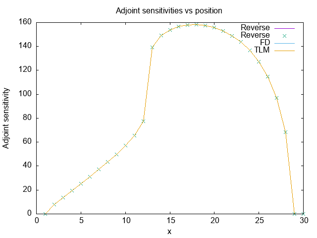
Fig. 8.2 xxb vs x for all methods used to calculate the sensitivities.
8.8.2.9. A note on Binomial Checkpointing
8.8.2.9.1. What is Checkpointing?
8.8.2.9.2. What is Binomial Checkpointing?
8.8.2.9.3. How to use Binomial Checkpointing with Tapenade?
Using binomial checkpointing is extremely simple with Tapenade. First we add the following line just before our time loop starts.
!$AD BINOMIAL-CKP nt+1 20 1
do t = 1,nt
    !!!! Stuff inside the time loop.
end do
Notice that for the fortran compiler the line we just added is a comment, but when Tapenade parses the code, it knows it needs to use binomial checkpointing. The line essentially tells Tapenade the following - “Use binomial checkpointing for this loop which has nt+1 steps (if you count the exit iteration as well), checkpoint every 20 steps, with the first step numbered as 1.” Tapenade uses some subroutines whose names start with ADBINOMIAL to manage the checkpointing and thus we need to link to the adBinomial.c file in the Makefile so that we tell the compiler what these subroutines are. (Essentially the same thing we did with adStack.c.)