7.2. Oceanic forcing
7.2.1. Sea level
The sea level surrounding the simulated ice sheet determines the land area available for glaciation. The level \(z=0\) corresponds to the mean sea level at present day, and the SICOPOLIS variable z_sl denotes the sea level relative to this reference.
Two different options for prescribing the sea level are available, selected in the run-specs headers by the parameter SEA_LEVEL:
1: Temporally constant sea level z_sl, specified by the parameterZ_SL0.3: Time-dependent sea level (e.g., reconstruction from data) from an input file (ASCII or NetCDF), specified by the parameterSEA_LEVEL_FILE.
Both options assume a spatially constant sea level. However, the variable z_sl is actually a 2D field, so that SICOPOLIS can handle in principle a spatially variable sea level as well.
7.2.2. Ice-shelf basal melting
The parameter FLOATING_ICE_BASAL_MELTING in the run-specs headers allows specifying the melting rate under ice shelves (floating ice), \(a_\mathrm{b}\). For all terrestrial ice sheets, the following options can be chosen:
1: Constant values for the continental shelf (\(a_\mathrm{b}^\mathrm{c.s.}\)) and the abyssal ocean (\(a_\mathrm{b}^\mathrm{a.o.}\)), respectively:(7.5)\[\begin{split}a_\mathrm{b} = \left\{ \begin{array}{ll} a_\mathrm{b}^\mathrm{c.s.} & \mbox{if}\;\; z_\mathrm{l} > z_\mathrm{abyss}\,, \\ a_\mathrm{b}^\mathrm{a.o.} & \mbox{if}\;\; z_\mathrm{l} \le z_\mathrm{abyss}\,, \end{array} \right.\end{split}\]where \(z_\mathrm{l}\) is the seabed (lithosphere surface) elevation and \(z_\mathrm{abyss}\) the threshold seabed elevation that separates the continental shelf from the abyssal ocean. The parameters \(a_\mathrm{b}^\mathrm{c.s.}\), \(a_\mathrm{b}^\mathrm{a.o.}\) and \(z_\mathrm{abyss}\) can be set in the run-specs headers (
QBM_FLOAT_1,QBM_FLOAT_3andZ_ABYSS, respectively).4: Local parameterization as a function of the oceanic thermal forcing \(T_\mathrm{f}=T_\mathrm{oc}-T_\mathrm{b}\) (difference between the ocean temperature \(T_\mathrm{oc}\) and the ice-shelf basal temperature \(T_\mathrm{b}\)):(7.6)\[a_\mathrm{b} = \Omega\,T_\mathrm{f}^\alpha\,.\]The parameters \(T_\mathrm{oc}\), \(\Omega\) and \(\alpha\) can be set in the run-specs headers (
TEMP_OCEAN,OMEGA_QBMandALPHA_QBM, respectively). The ice-shelf basal temperature is computed as(7.7)\[T_\mathrm{b} = -\beta_\mathrm{sw} d - \Delta{}T_\mathrm{m,sw}\,,\]where \(d\) is the draft (depth of the ice-shelf base below sea level), \(\beta_\mathrm{sw}=7.61\times{}10^{-4}\,\mathrm{K\,m^{-1}}\) the Clausius-Clapeyron gradient and \(\Delta{}T_\mathrm{m,sw}=1.85^\circ\mathrm{C}\) the melting-point lowering due to the average salinity of sea water.
For the Antarctic ice sheet, two additional options are available:
5: Sector-wise, local parameterization as a function of the thermal forcing (Greve and Galton-Fenzi [34]). This parameterization is modified after Beckmann and Goosse [4], with a linear dependence on the thermal forcing \(T_\mathrm{f}\) and an additional power-law dependence on the draft \(d\):(7.8)\[a_\mathrm{b} = \frac{\rho_\mathrm{sw}c_\mathrm{sw}\gamma_\mathrm{t}}{\rho L} \,\Omega\,\bigg(\frac{d}{d_0}\bigg)^\alpha \,T_\mathrm{f}\,,\]where \(\rho\) and \(\rho_\mathrm{sw}\) are the ice and sea-water densities, \(L\) is the latent heat of melting (all defined in the run-specs header), \(c_\mathrm{sw}=3974\,\mathrm{J\,kg^{-1}\,K^{-1}}\) is the specific heat of sea water, \(\gamma_\mathrm{t}=5\times{}10^{-5}\,\mathrm{m\,s^{-1}}\) is the exchange velocity for temperature and \(d_0=200\,\mathrm{m}\) is the reference draft.
The parameters \(\Omega\) and \(\alpha\) result from a tuning procedure for eight different sectors, using observed present-day melt rates as a target (as explained in the main part and appendix of Greve and Galton-Fenzi [34]). For the thermal forcing \(T_\mathrm{f}\), \(T_\mathrm{oc}\) is chosen for each sector as the sector-averaged temperature at 500 metres depth just outside the ice-shelf cavity (computed with data from the World Ocean Atlas 2009 [48]), while \(T_\mathrm{b}\) is computed by Eq. (7.7).
6: “ISMIP6 standard approach”: Sector-wise, non-local quadratic parameterization for the 18 IMBIE-2016 sectors (Rignot and Mouginot [55], The IMBIE Team [63]), where the two sectors feeding the Ross ice shelf and the two sectors feeding the Filchner–Ronne ice shelf are combined, leaving 16 distinct sectors (Jourdain et al. [43], Seroussi et al. [58]). The parameterization depends on the local thermal forcing \(T_\mathrm{f}\) and the sector-averaged thermal forcing \(\langle{}T_\mathrm{f}\rangle{}_\mathrm{sector}\) as follows:(7.9)\[a_\mathrm{b} = \gamma_0 \bigg(\frac{\rho_\mathrm{sw}c_\mathrm{sw}}{\rho L}\bigg)^2 \, (T_\mathrm{f} + \delta{}T_\mathrm{sector}) \, |\langle{}T_\mathrm{f}\rangle{}_\mathrm{sector} + \delta{}T_\mathrm{sector}|\,,\]where \(\rho\), \(\rho_\mathrm{sw}\), \(L\) and \(c_\mathrm{sw}\) are defined as in Eq. (7.8). The coefficient \(\gamma_0\), similar to an exchange velocity, and the sectorial temperature offsets \(\delta{}T_\mathrm{sector}\) are obtained by calibrating the parameterization against observations (see Jourdain et al. [43]).
The thermal forcing at the ice–ocean interface is derived by extrapolating the oceanic fields from GCMs into the ice-shelf cavities. Following the ISMIP6-Antarctica protocol, it must be provided as NetCDF input files that contain for each year the mean-annual, 3D thermal forcing for the entire computational domain. Thereby, this option allows prescribing a time-dependent thermal forcing (which is currently not the case for the other options). For the detailed parameter settings, see the description in the run-specs headers.
For all cases, an additional scaling factor \(S_\mathrm{w}\) can be applied (\(a_\mathrm{b}\rightarrow{}S_\mathrm{w}\,a_\mathrm{b}\)), defined as
This factor reduces the melting rate close to the grounding line where the water column \(H_\mathrm{w}\) is thin. The parameter \(H_\mathrm{w,0}\) can be set in the run-specs headers (H_W_0). A value recommended by Asay-Davis et al. [2] is \(75\,\mathrm{m}\), while Gladstone et al. [17] used \(36.79\,(=100/e)\,\mathrm{m}\). Setting this parameter to zero results in \(S_\mathrm{w}=1\) everywhere; the scaling is then switched off.
7.2.3. Ice-shelf calving
The options for calving of ice shelves (floating ice) can be selected in the run-specs headers by the parameter ICE_SHELF_CALVING:
1: Unlimited expansion of ice shelves, no calving.2: Instantaneous calving of ice shelves if the thickness is less than a threshold thickness, specified by the parameterH_CALV.3: “Float-kill”: Instantaneous removal of all floating ice.
For the Antarctic ice sheet, yearly ISMIP6-type ice-shelf collapse masks can be prescribed (Seroussi et al. [58]). This requires the setting ICE_SHELF_COLLAPSE_MASK = 1 and additional parameters as described in the run-specs headers.
7.2.4. Marine-ice calving
For calving of grounded marine ice, the following options are available:
Parameterization for “underwater-ice” calving (Dunse et al. [15]), to be selected by the following combination of run-specs-header parameters:
MARGIN = 2,MARINE_ICE_FORMATION = 2,MARINE_ICE_CALVING = 9. This parameterization is an adaption of the law by Clarke et al. [14], but acts here as an additional surface ablation rather than calving at a vertical front:(7.11)\[Q_\mathrm{c} = k_\mathrm{c} H^{r_1} D_\mathrm{w}^{r_2}\,,\]where \(Q_\mathrm{c}\) is the calving flux, \(H\) the ice thickness (taken to some power \(r_1\)), \(D_\mathrm{w}\) the water depth (taken to some power \(r_2\)) and \(k_\mathrm{c}\) the calving parameter (see also Fig. 7.3). The two exponents and the calving parameter can be set in the run-specs headers as parameters
R1_CALV_UW,R2_CALV_UWandCALV_UW_COEFF, respectively.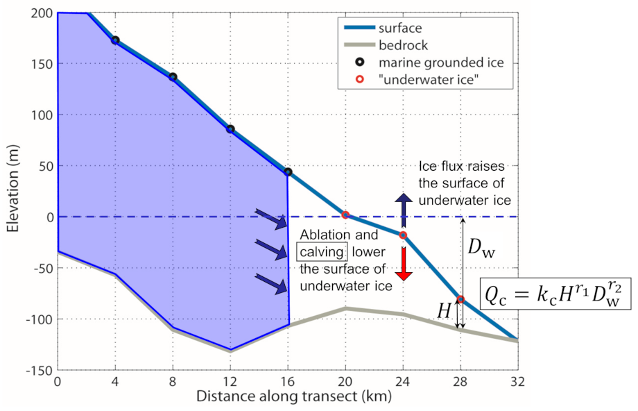
Fig. 7.3 Schematic of underwater ice calving. The purple area marks the marine grounded ice, the white area the “underwater ice” (fulfilling the floating condition) for which the calving law (Eq. (7.11)) is applied.
For the Greenland ice sheet, yearly ISMIP6-type retreat masks can be prescribed (Goelzer et al. [19]). This requires the setting RETREAT_MASK = 1 and additional parameters as described in the run-specs headers.